Picking OBS data with the Kingdom Suite
- There were problems with this method in TKS 7.2. 7.1 and newer (>=7.3) versions of TKS work properly again.
- OBS Data setup:
- The SEGY must be in the standard IBM format, and have monotonically incrementing trace numbers, otherwise the display may have data gaps. Dalhousie OBS data seem to display this problem, but it is easily fixed by the use of Claritas modules MISSING and SETHEADER. This is described in ObsSegyProcessing.
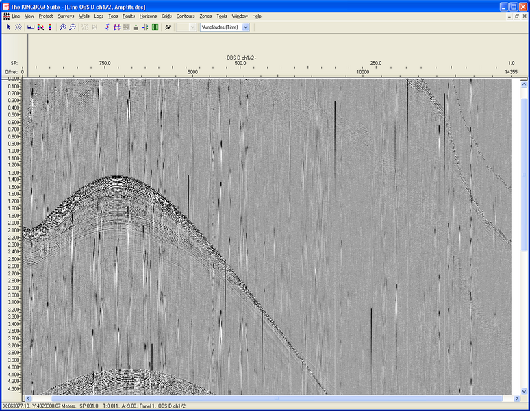
- Import 2d SEGY into TKS. This is an intuitive process. True coordinates are needed if you want to display the data with offset information. Coordinate information in 'traceNum degrees minutes decimal minutes' or 'traceNum UTMX UTMY' (space delimited) seems to work the best. The following figure shows some high resolution OBS data imported into TKS (its badly aliased).

- If you have more than one channel of data (hydrophone and geophone data from the same instrument, for example), these can both be picked in the same window. Simply import the second Segy file, and instead of creating a new 2d survey, select the same survey as before and create a new attribute (eg: 'geophone'). Now you can switch between the hydrophone and the geophone(s) in the same window. This is very useful as it allows the user to select the best channel for picking a desired phase.
- The SEGY can now be displayed on screen, and you can start digitizing (picking) if you like. However, this becomes Very difficult because of the moveout of the OBS data. This can be corrected with a Reduction Velocity (LMO static correction) or a Normal Moveout Correction (NMO static correction).
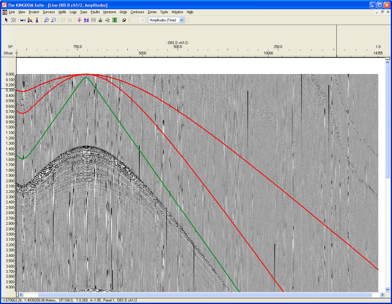
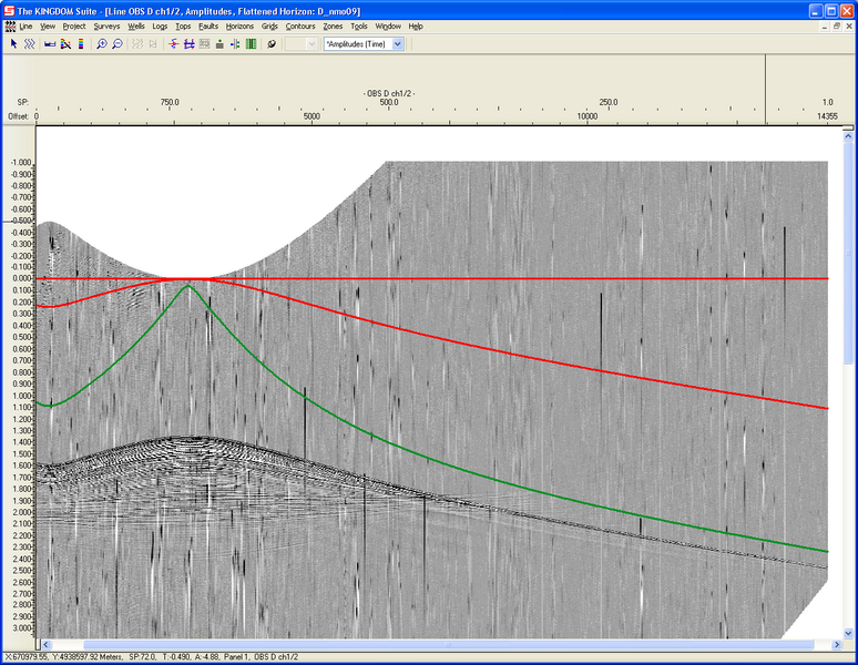
- Run the following python program »upload/segyinfo2horizon.py. It will create a bunch of individual files containing 'lineName trace time' info for each LMO and NMO curve defined. Run './segyinfo2horizon.py -h' to see the help for the program. Basically the program will read trace number and offset information from an input file (TRPRINT output from Claritas, the tempheader output from SeisWide, or a shottable) and write out several files containing curves for LMO and NMO curves. Flattening the OBS data in TKS with these curves makes it much easier to pick weak phases to far offsets.
- If the data is clipped on the top or bottom while the horizon is flattened, click on the settings icon (3rd from the left on the seismic window). Click on the Vert. Scale tab, and increase the values for Offset Time(s) (above and below). This will display the data you wish to see.
- Another useful function in TKS are filters. Bandpass filters can be applied 'on the fly', without the need to reload anything. This can be useful for phase identification, when it may be obscured by data of another frequency.
- Now that the phases are relatively easy to identify, you can pick them as horizons. The picking parameters are useful and powerful, but the 2d fill or manual pick are usually the best. Name the phases with with appropriate names, because they are exported alphanumerically. Therefore it makes sense to have the direct wave exported first (eg: reflPhase01, reflPhase02, reflPhase03, etc.).
- If the pick are satisfactory, they can be exported to many formats. Choose the geoquest card image if you wish to export all the horizons into one file (a good idea). This can be converted to a Rayinvr compatible 'tx.in' format with the program »upload/geoquest2zelt.py. This surprisingly complex program has several options for handling reduction velocities, time shifts, and output formats.
- Once the 'tx.in' file is output, analysis with Rayinvr can begin. However, it is likely that the picks will have to be refined several times.
- See RayinvrExampleA for a very quick introduction to the use of Rayinvr for OBS data.
- This shows the basic unfiltered OBS data (hydrophone)

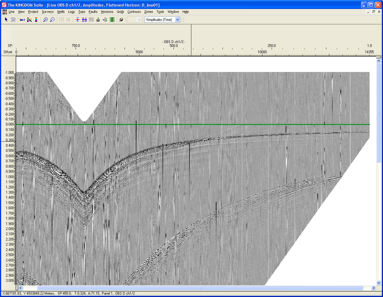
- Here is what an imported LMO horizon looks like (good for picking refracted phases):

- Here is what the data looks like when the LMO horizon is flattened:

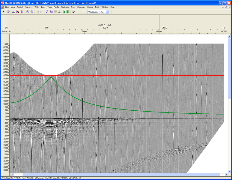
- The red curve (horizon) is an NMO curve.

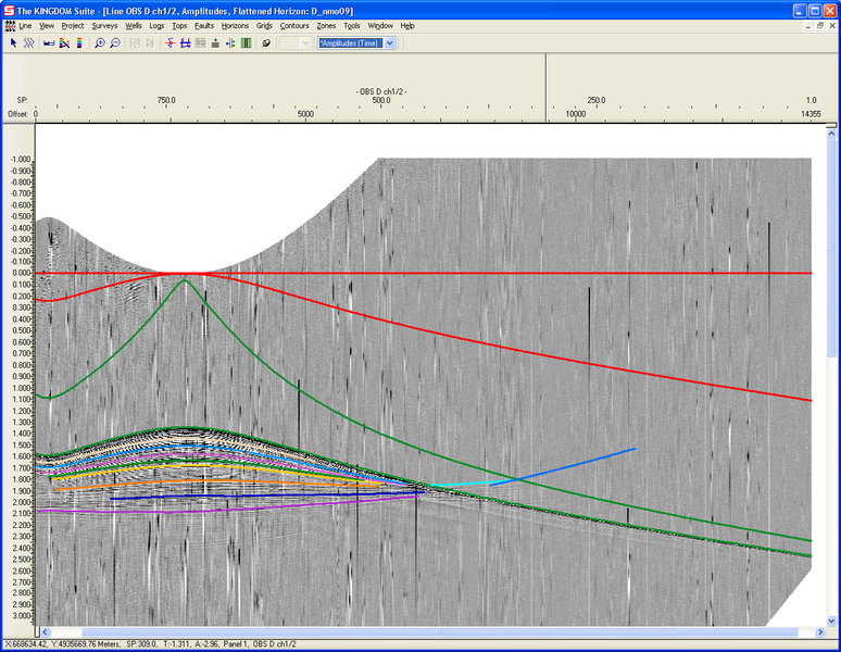
- The NMO curve is now flattened. The correct velocity and depth have been chosen to flatten the direct arrival.

- Another NMO curve has been imported which is at a higher velocity and depth, which will flatten a deeper reflected arrival (next figure).

- The deeper reflected arrival flattened by the last curve imported. It is much easier to identify the arrivals to far offset with this approach:

- This image shows 9 reflected and 2 refracted phase picks.
